Electronic properties of isolated molecules

Prev:LabQSM#Module 2: DFT simulations of Molecules (6h)
Calculation of molecules: Intro

At variance with bulk crystalline systems (fully periodic in 3D), molecules are finite isolated systems, and special care needs to be put in setting up calculations, accordingly.
- scf + nscf: DFT calculations for molecules (or systems with reduced dimensionality in general) follow the same strategies discussed in the previous lectures, where scf calculations are followed by nscf runs (and perhaps by post-processing steps, as discussed below in Electronic properties of isolated molecules#Post processing tools).
- isolation: when localised basis sets are used, systems are usually treated as isolated by default (and care must be used to impose periodicity). Instead, when using plane-waves, periodic boundary conditions (PBC) are automatically enforced and molecule isolation has to be imposed.
- vacuum: As a preliminary step, the unit cell describing an isolated molecule has to be large enough to avoid direct chemicalinteraction (ie chemical bonds) of atoms belonging to different replicas (given PBC, the atoms in one cell are infinitely repeated, giving rise to a lattice of replicas).
- electrostatics: similarly, one also wants to avoid electrostatic interactions (driven in Kohn-Sham DFT by the Hartree potential) among replicas. The presence of long range interactions (dipoles, quadrupoles...) makes convergence wrt vacuum (ie cell size) slow and dedicated techniques should be used. When using Quantum ESPRESSO, consider setting
assume_isolated="mt"(standing for Martyna Tuckerman approach, as from J. Chem. Phys. 110, 2810 (1999)) in theSYSTEMnamelist. - When charged systems are considered the situation is even more critical: in principle the total energy would diverge for a system in PBC, and by default a compensating uniform background is added to the system (though resulting in spurious effects in the properties of the system). In this cases the use of the Martyna-Tuckerman approach is strongly recommended.
- In principle, the exchange-correlation energy and potential would also have a contribution related to the presence of replicas (long range physical contributions are also there, just consider van der Waals interactions as an example). Nevertheless, when using simple approximations to the xc functional (eg LDA, GGA, meta-GGA) long range contributions are not present and so the xc term does not pose any problems.
- Overall, a 10-15 Angstrom of vacuum in between replicas is typically enough to describe neutral molecules with mild dipoles to a decent accuracy. If the Martyna-Tuckerman approach is used, one needs to be very careful with the molecule separation since it needs to be at least as large as the physical dimension of the system in that direction (so for elongated molecules a large region of vacuum is actually needed).
- Importantly: though rules of thumb exist (see above), the amount of vacuum to be included in the system description is a convergence parameter that needs to be tested against the quantities of interested to be calculated.
K-points and Gamma sampling
- The Brillouin zone of a infinitely large cell subject to PBC becomes a single point, Gamma. Because of this, even when using a large but finite cell, K-point sampling should not be used. This should not be relevant in terms of results (if it is, spurious interactions are present), but would result in a waste of computational resources. The so-called Gamma sampling should then be sued.
- Moreover, in view of the Gamma sampling, wave functions can be taken to be real, leading to more memory and computational time savings.
- In Quantum ESPRESSO one needs to set the following:
  K_POINTS automatic
  1 1 1   0 0 0         # for Gamma sampling using complex wavefunctions
                        # deprecated, unless for testing or debugging
K_POINTS (gamma) # for proper gamma sampling using real wavefunctions
Post processing tools
Here we take the occasion to introduce some among the post processing tools of Quantum ESPRESSO.
By post processing (PP) one means the set of tools and operations to be performed on the output data of the calculations (here the simulations performed at the DFT level). Quantum ESPRESSO provides a tool, pp.x, dedicated to post-processing calculations.
Possible quantities that can be extracted and plotted using pp.x:
- charge density
- electrostatic potential (V_ion + V_H)
- total Kohn-Sham potential (V_ion + V_H + V_xc)
- selected Kohn-Sham orbitals
Here is an example input file (pp.in):
 &INPUTPP
    prefix="..."
    outdir="..."
    plot_num=11            # electrost. Pot
    filplot = "pot.pp"
 /

 &PLOT
    nfile=1
    filepp(1)="pot.pp"
    iflag=3
    output_format=5        # xsf xcrysden fmt
    fileout="pot.xsf"
 /
where plot_num can be chosen according to:
 plot_num =
   0      total charge
   1      total potential
   5      STM images
   7      KS orbitals
  11     electrostatic potential
Usage:
[mpirun -np num_mpi_tasks] pp.x < pp.in > pp.out
More options are available at: INPUT_PP
Another post-processing tool useful in this context is average.x which performs
a planar average of a given input scalar field on a 3D grid. Additionally, a double average (convolution with a rolling window)
is also performed.
This is particularly useful, e.g., to plot the average potential, in the form v(z), in the vacuum region of the cell
in order to determine the position of the vacuum level. See exercises for more details.
An example of an input file (average.in) follows:
 1           # nfile
 pot.pp      # filename
 1.0         # weight
 96          # n-points (FFT mesh)
 3           # idir
 1.0         # awin  (width of the rolling window)
Usage:
average.x < average.in
Exercises
Exercise 1


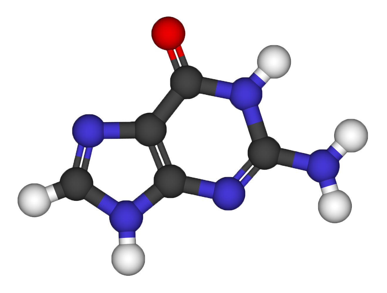
Structural relaxation of the Guanine molecule
- Use a molecular builder to find the initial molecular structure. (Avogadro)
- Perform classical force field (FF) relaxation (using a built-in engine)
- Setup a DFT calculation with the guanine structure obtained from Avogradro (check both the amount of vacuum and the kinetic energy cutoff to be used)
- Perform a quantum mechanical (DFT based) refinement of the relaxation (using Quantum ESPRESSO, with thr=10^-3 on forces)
- Use the xcrysden software to visualize the relaxation path.
Exercise 2
Electronic properties of the Guanine molecule
Using the guanine atomic coordinates determined at the previous step, compute:
- HOMO and LUMO frontier orbital energies
- How do they depend on the supercell volume and why?
- Estimate the vacuum level wrt supercell size (pp.x, average.x)
- Repeat the calculation using the “assume_isolated” variable
- Is -HOMO a good estimate of IP ? IP_exp=8.0-8.3 eV
Janak's theorem, Piece-wise Linearity, Ionization potential
Here we try to rationalise the numerical results obtained so far in the evaluation of the ionisation potential as negative of the HOMO eigenvalue.
A first important result is related to Janak's theorem, Phys. Rev. B 18, 7165 (1978), stating that:
 dE[n]/df_i = eps_i    where
 n(r) = sum_i f_i * |psi_i(r)|^2
i.e, the derivative of the total energy wrt a fractional occupation of the i-th orbital equals the i-th eigenvalue. As a total derivative, this makes sense when considering the occupation of the HOMO and gives a physical meaning to the HOMO eigenvalue.
The total energy can also be extended to fractional number of electrons (making a statistical mixture of systems at N and N-1 electrons), and should be piece-wise linear (PWL).
The ionisation potential is defined as
IP = E[N-1] -E[N]
Computing the IP following the above expression takes the name of Delta-scf.
Because of Janak's theorem, one should also have:
IP = -eps_HOMO
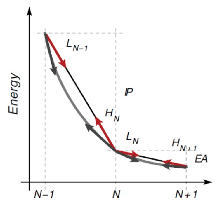
While the two methods should give the same result in exact KS-DFT, when approximate functionals are used this is no longer true. In particular, the total energy is no longer piece-wise-linear but convex (for standard local and semi local functionals). This is depicted in the figure below.

Here the slope of the PWL total energy curve between N-1 and N electrons correspond to the IP computed as a finite difference of total energy. Instead the slope at integer occupations corresponds to the negative of the HOMO eigenvalue.
When convexity due to, e.g., LDA or PBE, is present, the HOMO eigenvalue turns out to be less negative (i.e. higher in energy) than it should. Viceversa for the LUMO (too deep). These behaviours are also connected to an over-delocalization (then leading eg also to over-hybridisation) error of the orbitals and of the charge density.
For a review on the topic see: L. Krnoik and S: Kummel Piecewise linearity, freedom from self-interaction, and a Coulomb asymptotic potential: three related yet inequivalent properties of the exact density functional. Phys. Chem. Chem. Phys. 22, 16467 (2020)
Exercises
Exercise 3
Electronic properties of the Guanine molecule
What does IP mean? [ IP = Etot(N-1)-Etot(N) ]
- Let’s do this calculation explicitly (the ∆-scf procedure)
- Repeat the calculation for different volumes
- Repeat the above using different functionals (LDA,PBE,PBE0,HF...).
Note: hybrid functionals may take very long, special care must be used in setting the parameters
Exercise 4
Electronic properties of the Guanine molecule
- Density, HOMO and LUMO orbitals and plot them (pp.x + xcrysden)
- How do the HOMO and LUMO orbitals look like?
- Density of states (dos.x tool)
- The projected density of states (projwfc.x tool + sumpdos.x)
Exercise 5
A simple Reaction: Methane Combustion


Calculate the reaction Enthalpy of the methane combustion:
CH4+2O2 → 2H2O+CO2
EXP: ∆Hc = -890 KJ/mol = 212.7151051 Kcal/mol
H = U + pV
∆Hc = Etot(products) -Etot(reactants) (at std p,T)
because : p∆V = ∆n R T and ∆n=0
- Relax and calculate tot energies for all the reactants and products using the template input
- Starting atomic coordinates of the molecules are in ./LAB_2/docs/g2-97_cart_neut.txt
- Pay attention to the O2 molecule (triplet)