Structural and electronic properties of semiconductors and metals
Prev: LabQSM#Lecture 1: Basic DFT calculations and Convergences
Structural and electronic properties of Diamond

In this tutorial we will see how to setup a calculation and to get total energies using the PW code from the Quantum ESPRESSO distribution.
Some helpful conversions:
1 Bohr = 1 a.u. (atomic unit) = 0.529177249 Angstroms.
1 Rydberg  = 13.6056981 eV
1 eV =1.60217733 x 10^-19 Joules
For all first-principles calculations, you must pay attention to two convergence parameters. The first one is the energy cutoff, which is the max kinetic energy used in wave-function expansion. The second is the number of k-points, which measures how well the continuous integral over the BZ is discretized.

Diamond is a face-centered cubic structure with two C atoms at 0 0 0 and 0.25 0.25 0.25 a is the lattice parameter
Now let's see in detail how a QE input is structured to make a total energy calculation for this system. An example can be found in ~/LabQSM/LAB_1/test_diamond/scf.diamond.in that you can read e.g. using the editor vi:
Input file description
&CONTROL
   prefix='diamond',
   calculation = 'scf'
   restart_mode='from_scratch',
   pseudo_dir = './pseudo/'
   outdir = './SCRATCH'
/
&SYSTEM
   ibrav = 2,
   celldm(1) = 6.7402778
   nat = 2,
   ntyp = 1,
   ecutwfc =  40.0
/
&ELECTRONS
   mixing_mode = 'plain'
   mixing_beta = 0.7
   conv_thr =  1.0d-8
/
ATOMIC_SPECIES
 C   12.011   C.pz-vbc.UPF
ATOMIC_POSITIONS (alat)
 C 0.00 0.00 0.00
 C 0.25 0.25 0.25
K_POINTS {automatic}
 4 4 4   0 0 0
The input file for PWscf is structured in a number of NAMELISTS and INPUT CARDS:
&NAMELIST1 ... /
&NAMELIST2 ... /
&NAMELIST3 ... /
INPUT_CARD1
 ....
 ....
INPUT_CARD2
....
....
The use of NAMELISTS allows to specify the value of an input variable, not all the variables need to be specified, for most variable, a default value is assigned. Variable can be inserted in any order. NAMELISTS are read in a specific order. INPUT CARDS are specific of QuantumESPRESSO codes and are used to provide input data that are always needed.
There are three mandatory NAMELISTS (while more can be required according to the calculation type):
- &CONTROL: variables that control the kind of calculation (here scf), where to get the pseudopopotentials, and the verbosity needed in the output.
- &SYSTEM: variables specifying the system as the crystal structure, number of atoms, dimension of the basis set.
- &ELECTRONS: variables controlling the algorithm to solve the Kohn-Sham equations.
- &IONS: needed only for some values of the
calculationvariable (CONTROL namelist), such as set to "relax" or "vc-relax". - &CELL: as above, needed for selected kind of calculations, including "vc-relax".
Next, we have three mandatory INPUT CARDS:
- ATOMIC_SPECIES : name, mass and pseudopotential file
- ATOMIC_POSITIONS: atom type and coordinate in the unit cell
- K_POINTS: definition of the k point grid for the BZ integration
Other NAMELISTS relative to other kinds of calculations as relaxations, cell relaxations and other INPUT CARDS will be shown later.
The complete list of QE variables can be found in the documentation of the code at: | http://www.quantum-espresso.org/Doc/INPUT_PW.html
Now that we know how a QE input looks like let's run it and see what the code does and analyze the output:
Running pw.x
Let's create a working directory e.g.
$> mkdir diamond
and copy in this directory the scf.diamond.in input file we have inspected.
Now you can run the pw.x executable as:
$> pw.x < scf.diamond.in > scf.diamond.out
It is also possible to run in parallel:
$>  export OMP_NUM_THREADS=2       #we use 2 OpenMP threads
$>  pw.x < scf.diamond.in > scf.diamond.out
or
$> mpirun -np 2 pw.x < scf.diamond.in > scf.diamond.out #we use 2 MPI tasks running on 2 processors
Several files will be generated in ./SCRATCH, most of them needed mainly for post-processing now let's have a look to the readable output (scf.diamond.out).
Output file description:
Bearing in mind the logical flow of a self-consistent Kohn-Sham DFT calculation performed using the density mixing approach, defined in the figure,
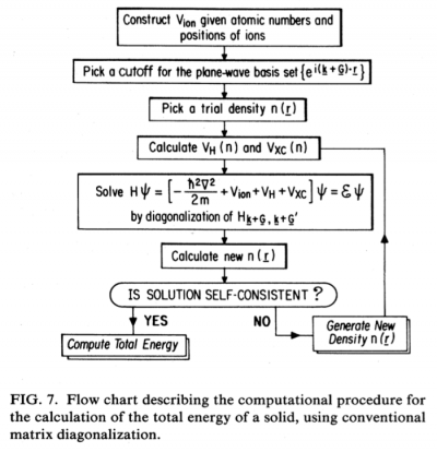
we can now inspect the output (scf.diamond.in > scf.diamond.out) using the vi/more/less command.
This is what we find:
A recap of the configuration that is being calculated:
    bravais-lattice index     =            2
    lattice parameter (alat)  =       6.7403  a.u.
    unit-cell volume          =      76.5550 (a.u.)^3
    number of atoms/cell      =            2
    number of atomic types    =            1
    number of electrons       =         8.00
    number of Kohn-Sham states=            4
    kinetic-energy cutoff     =      40.0000  Ry
    charge density cutoff     =     160.0000  Ry
    convergence threshold     =      1.0E-08
    mixing beta               =       0.7000
    Exchange-correlation=  SLA  PZ   NOGX NOGC
Detailed information of the unit cell:
   celldm(1)=   6.740278  celldm(2)=   0.000000  celldm(3)=   0.000000
   celldm(4)=   0.000000  celldm(5)=   0.000000  celldm(6)=   0.000000
   crystal axes: (cart. coord. in units of alat)
              a(1) = (  -0.500000   0.000000   0.500000 )
              a(2) = (   0.000000   0.500000   0.500000 )
              a(3) = (  -0.500000   0.500000   0.000000 )
   reciprocal axes: (cart. coord. in units 2 pi/alat)
              b(1) = ( -1.000000 -1.000000  1.000000 )
              b(2) = (  1.000000  1.000000  1.000000 )
              b(3) = ( -1.000000  1.000000 -1.000000 )
Information on the used pseudopotential:
 PseudoPot. # 1 for C  read from file:
    /home/max/LabQSM/pseudo/C.pz-vbc.UPF
    MD5 check sum: ab53dd623bfeb79c5a7b057bc96eae20
    Pseudo is Norm-conserving, Zval =  4.0
    Generated by new atomic code, or converted to UPF format
    Using radial grid of  269 points,  1 beta functions with:
               l(1) =   0
    atomic species   valence    mass     pseudopotential
       C              4.00    12.01100     C ( 1.00)
Information on the symmetries operation detected
48 Sym. Ops., with inversion, found (24 have fractional translation)
Information on the k points used to sample the Brillouin zone and FFT gird:
number of k points=     8
                      cart. coord. in units 2pi/alat
       k(    1) = (   0.0000000   0.0000000   0.0000000), wk =   0.0312500
       k(    2) = (  -0.2500000   0.2500000  -0.2500000), wk =   0.2500000
       k(    3) = (   0.5000000  -0.5000000   0.5000000), wk =   0.1250000
       k(    4) = (   0.0000000   0.5000000   0.0000000), wk =   0.1875000
       k(    5) = (   0.7500000  -0.2500000   0.7500000), wk =   0.7500000
       k(    6) = (   0.5000000   0.0000000   0.5000000), wk =   0.3750000
       k(    7) = (   0.0000000  -1.0000000   0.0000000), wk =   0.0937500
       k(    8) = (  -0.5000000  -1.0000000   0.0000000), wk =   0.1875000
Dense grid: 2685 G-vectors FFT dimensions: ( 20, 20, 20)
Here note that the 2685 G-vectors are defined, using the ecutrho variable, as points inside a cutoff sphere in reciprocal space. The FFT grid, mapping direct to reciproca space, is built as a box containing the cutoff sphere.
Intermediate energies calculated during the scf loop
Self-consistent Calculation
    iteration #  1     ecut=    40.00 Ry     beta= 0.70
    Davidson diagonalization with overlap
    ethr =  1.00E-02,  avg # of iterations =  2.0
total cpu time spent up to now is 0.2 secs
    total energy              =     -22.67865569 Ry
    Harris-Foulkes estimate   =     -22.74103732 Ry
    estimated scf accuracy    <       0.12254037 Ry
...
Near the end “hopefully” our converged results
Final Eigenvalues for each k point:
End of self-consistent calculation
k = 0.0000 0.0000 0.0000 ( 331 PWs) bands (ev):
-8.0812 13.3868 13.3868 13.3868
k =-0.2500 0.2500-0.2500 ( 323 PWs) bands (ev):
-6.3642 6.7040 11.6380 11.6380
For each k-point, the number of G-vectors used to represent the wave functions are provided
(331, 323, ...). These are k-dependent (the cutoff sphere for wave function is defined on k+G vectors and is therefore k-dependent).
When ecutrho = 4* ecutwfc (as it should for nota-conserving pseudopotentials), the number of G-vectors in the density grid is almost 8 times
that of G-vectors in the wfc grid (geometrically, the kinetic energy cutoff is the square of the sphere radius, the number of G-vectors being proportional to its volume).
Final total energy and contribution of the various terms:
Note that the converged total energy is preceded by an exclamation mark "!".
!   total energy              =     -22.68935940 Ry
    Harris-Foulkes estimate   =     -22.68935940 Ry
    estimated scf accuracy    <          1.5E-09 Ry
The total energy is the sum of the following terms:
    one-electron contribution =       8.08269762 Ry
    hartree contribution      =       1.85703398 Ry
    xc contribution           =      -7.05484267 Ry
    ewald contribution        =     -25.57424832 Ry
convergence has been achieved in 6 iterations
At the end of the file, you can find info on timings spent in each part of the code (subroutines):
PWSCF : 0.13s CPU 0.32s WALL
Now we can, for instance, extract the total energy calculated at each step of the self-consistent loop:
$>grep -e "total energy" scf.diamond.out
or the accuracy reached AT each step:
$> grep -e "scf" scf.diamond.out
or we can grep both of them and put in a two-column format:
$> grep -e "total energy" -e "scf" scf.diamond.out | awk '/l e/{e=$(NF-1)}/ scf / {print e, $(NF-1)}'
-22.67865569 0.12254037
-22.68899239 0.00212159
-22.68934113 0.00007686
-22.68935832 0.00000263
-22.68935938 0.00000004
-22.68935940 1.5E-09
or we can redirect to a file to be plot
$> grep -e "total energy" -e "scf" scf.diamond.out | awk '/l e/{e=$(NF-1)}/ scf / {print e, $(NF-1)}' > diamond_scf.dat
$> gnuplot
$> plot "diamond_scf.dat" u 0:1 wlp
$> p "diamond_scf.dat"  u 0:(log10($2)) w lp  ,-8
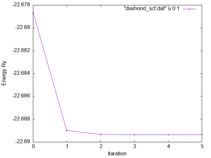
Total Energy vs iteration
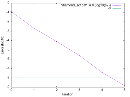
Relative error vs iteration


Exercises
Exercise 1
Parsing pw output files
- Write a script to extract the total energy and the lattice parameter from a pw output file
- Print them on the same output line
- Solve the problem using a bash script (e.g. called
extract.sh) - Try to do the same also using a awk script (
extract.awk) - If you are a python expert you can give it a try (
extract.py)
Note that .sh and .py scripts can be made easily working on multiple files
- Hint1: the total energy is marked by "!", while the lattice parameter can be taken from celldm1 (marked by "lattice parameter")
- Hint2: look at an example and build the scripts checking step by step, use e.g. scf.diamond.out
Exercise 2
Convergence wrt k-points
- Using a script, perform different runs in order to converge the absolute energy of your system with respect to the k-point sampling
(keep other variables fixed).
- You can use a cutoff lower than the converged one (~40 Ry)
- Hint: Try 4x4x4, 6x6x6, 8x8x8 etc...
- Take also a look at the number of the irreducible k-points generated by the code and at the relative execution time.
Exercise 3
Convergence wrt wavefunction kinetic energy cutoff (ecutwfc)
- Using a script, perform different runs in order to converge the absolute energy of your system with respect to the plane waves kinetic energy cutoff used to represent the wave functions.
- Hint: Use an increment 20 Ry in the range 20-200 Ry;
- for the purpose of evaluating the scaling of time-to-solution wrt ecutwfc, you can push the calculations to even larger (and further unrealistic) values (such as 300 and 400 Ry).
- Convergence criteria ~5meV/atom
BTW: Note that this is NOT the procedure to follow to determine the kinetic energy cutoff to use in production runs.
In fact, values determined in this way tend to be much larger than the cutoff actually needed for most applications we are interested in.
Exercise 4
Convergence of Energy differences wrt ecutwfc
- Using a script, compute the energy difference corresponding to using two lattice parameters and perform several runs in order to converge such a difference with respect to the plane wave kinetic energy cutoff.
- Hint1: Use an increment of 20 Ry in the range 20-200 Ry
- Hint2: consider a variation of the lattice parameter providing a sensible energy difference (1-2% is ok)
- Convergence criteria: ~ 0.1 mRy/atom
- How does the convergence compare with the one of the bare total energy ?
Exercise 5
Convergence of forces wrt ecutwfc
- Displace a C atom by +0.05 (in alat or crystal relative coords) in the z direction to induce non-zero forces acting atoms (otherwise forbidden by symmetry).
- Keeping the other parameters fixed, calculate the forces on C as a function of the kinetic energy cutoff.
- A good threshold on force convergence is 1 to 0.1 mRy/Bohr.
Hint: Remember to set tprnfor=.true. in the namelist control.
Lattice parameter & Elastic constants
Here we briefly introduce some poor-man approaches to compute the lattice parameter and bulk modulus of simple crystals by directly evaluating total first and second derivatives wrt the lattice parameter.
We do this in the form of guided exercises.
Exercise 6
Lattice parameter of diamond
Structural Relaxation
This is a new runlevel of Quantum Espresso and it is aimed at mechanical stability: make total energy stationary wrt FORCES and components of the STRESS TENSOR. The code will perform a series of scf calculation moving ions or cell parameters until a convergence criterium is reached.
These kinds of calculation are activated selecting:
calculation=”relax” # cell is fixed
Or
calculation=”vc-relax” # variable-cell relax
and they need additional mandatory namelists which are:
- &IONS # cell is fixed, but atoms move: it will contain input variables that control the ionic motion dynamic in structural relaxation
- &CELL # the cell moves: it will contain variables that control the shell-shape dynamics in structural relaxation
Examples are:
&CONTROL
     [...]
     forc_conv_thr=1.0d-4
     etot_conv_thr=1.0d-5
/
[…]
&IONS
     ion_dynamics=”bfgs”
     [...]
/
&CELL
     cell_dynamics=”bfgs”
     press_conv_thr=0.5
     cell_dofree=”all”
     [...]
/
In this example, we used the BFGS quasi-newton algorithm for both cell dynamics and ion dynamics, and we are optimizing all axis and angles (cell_dofree=”all”), it is also possible to keep fixed some structural parameter fixed or insert constraints see cell_dofree options.
Exercise 7
Take a scf input file for diamond, offset one of the two atoms Set a initial lattice far from the equilibrium condition (eg -5%) Using “relax” and “vc-relax” find the optimum geometry Plot the resulting lattice parameter as a function of the kinetic energy cutoff