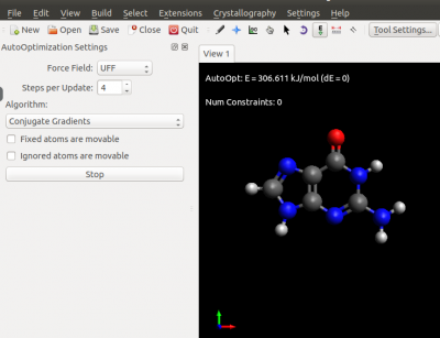
Solution LAB2 guanine
- Back to the previous page: Electronic properties of isolated molecules#Exercise 1
Step 1: geometry building
- Once you have Avogadro installed, open it and let's use the molecular builder to visualise a Guanine molecule:
Build --> Insert-->Fragment-->nucleobases-->guanine
Click on the selection settings "arrow" and right click to visualise the molecule.
Clicking on manipulate settings "hand" you can then rotate the molecule.
- Now we perform a classical relaxation using an Avogadro built-in Force Filed
 Extension-->Molecular Mechanics and we choose a FF
 Extension-->Optimize geometry
In few steps we have our relaxed geometry that we can save in .xyz format using:
File-->Save as-->select .xyz format and save in your disk as guanine_FF.xyz
The result of your FF optimisation should look like the following
Step 2
Now we are ready to perform a DFT simulations. As a first step, update your pseudo potentials directory by using git commands:
git pull
new pseudo potentials (Nitrogen and Oxygen) will be downloaded in your pseudo potential directory.
Create a scf input file (guanine_scf.in) paying attention to:
ibrav=8 #orthorombic cell with vacuum
celldm(1) = 25.00
celldm(2) =  1.0
celldm(3) =  0.8
Set the correct number and types of atoms. Set all the atomic species using the psuedo you have downloaded:
H   1.0  H.pz-vbc.UPF
C   1.0  C.pz-vbc.UPF
N   1.0  N.pz-vbc.UPF
O   1.0  O.pz-mt.UPF
insert the atomic positions in Angstrom:
ATOMIC_POSITIONS (angstrom)
Important:
- How many k-points you need?
- the amount of vacuum needs to be converged
- same for the kinetic energy cutoff (note that here we can use the value of the total force as a convergence parameter)
 # ecutwfc Ry
 40    Total force =     0.316709     Total SCF correction =     0.000067
 50    Total force =     0.315474     Total SCF correction =     0.000089
 60    Total force =     0.319550     Total SCF correction =     0.000100
 80    Total force =     0.322261     Total SCF correction =     0.000098
100    Total force =     0.323131     Total SCF correction =     0.000119
120    Total force =     0.323153     Total SCF correction =     0.000140
Despite 60-80 Ry seem to be appropriate, here we decide to use ecutwfc=50 in order to keep the calculation time under control.
Step 3
We can now run a QM relaxation using DFT. Edit the input file according to:
 &CONTROL
 [...]
 calculation="relax"
 etot_conv_thr=1.0D-4
 forc_conv_thr=1.0D-3
 # we set a medium-tight threshold in order not to have a too long calculation
 /
and add the &IONS namelist.
Run the relaxation, it will take a while to rearrange the atoms in the relaxed positions according to the threshold parameter.
$> pw.x < guanine_relax.in > guanine_relax.out &
One the job has converged you can compare the initial position (Force Field relaxed) with the final ones (QM relaxed). You can use xcrysden to visualise the optimisation steps.
xcrysden --pwo guanine_relax.out
you can reduce the dimensionality to 0D and choose the option: Display All Coordinates as Animation In this way you will have a movie of the molecule relaxation
