Solution LAB1 bands DOS diamond

• Back to the previous page: Structural and electronic properties of semiconductors and metals #Convergences

Band structure and DOS of Diamond

Given the calculations run previously to determine the converged set of k-points, ecutwfc, and lattice parameter, here we set the following:

 nk = 8
 ecutwfc = 60.0     # could be lowered further
 alat = 6.6694212

As a preliminary step:

• make a new directory, e.g. called Diamond_BANDS
• In a situation like this it is always a good idea to start over from scratch with a fresh scf calculation.
• prepare an input file for a single scf run according to the parameters above.

 &CONTROL
   calculation="scf"
   [...]
 /
 &SYSTEM
   alat=...
   ecutwfc=...
 /
 [...]
 K_POINTS {automatic}
 8 8 8  0 0 0

• run the calculation as:

 mpirun -np 2 pw.x < scf.in > scf.out

• The use of mpirun -np 2 in the example above makes the calculation running on two MPI processes.

We start by addressing the calculation of the DOS.

We need now to write the input file for a non-self consistent calculation using a regular k-point grid. The input file looks like:

 >$ cat nscf_dos.in
 &CONTROL
   calculation="nscf"
   verbosity="high"     # not strictly needed but useful sometimes
   [...]
 /
 &SYSTEM
   alat=...
   ecutwfc=...
   nbnd=20              # let's include some empty states
 /
 [...]
 K_POINTS {automatic}
 20 20 20  0 0 0        # here we use a much denser kpt grid

Then we run it

 mpirun -np 2 pw.x < nscf_dos.in > nscf_dos.out

Given the number of k-points requested, the calculation may take some time.

At this point we can prepare an input file for the dos.x program,

 $> cat  dos.in
 &DOS
    prefix = 'diamond'
    outdir = './SCRATCH/'    
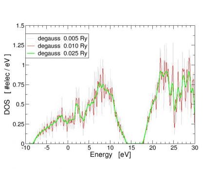
    degauss=0.025  !  [Ry]  broadening parameter
    fildos = 'dos_diamond_0.025Ry.dat'
 / 

The variable degauss controls the gaussian broadening used to approximate Dirac delta's in the calculation.

Try to change this value to get a feeling of the effect is has on the computed DOS.

An example is show in the figure below.