Solution LAB1 bands DOS diamond

• Back to the previous page: Non self-consistent calculations: Band structures and Density Of States#Examples and Exercises

Preliminaries

Given the calculations run previously to determine the converged set of k-points, ecutwfc, and lattice parameter, here we set the following:

 nk = 8
 ecutwfc = 60.0     # could be lowered further
 alat = 6.6694212

As a preliminary step:

• make a new directory, e.g. called Diamond_BANDS
• In a situation like this it is always a good idea to start over from scratch with a fresh scf calculation.
• prepare an input file for a single scf run according to the parameters above.

 &CONTROL
   calculation="scf"
   [...]
 /
 &SYSTEM
   alat=...
   ecutwfc=...
 /
 [...]
 K_POINTS {automatic}
 8 8 8  0 0 0

• run the calculation as:

 mpirun -np 2 pw.x < scf.in > scf.out

• The use of mpirun -np 2 in the example above makes the calculation running on two MPI processes.

DOS of Diamond

We start by addressing the calculation of the DOS.

We need now to write the input file for a non-self consistent calculation using a regular k-point grid. The input file looks like:

 >$ cat nscf_dos.in
 &CONTROL
   calculation="nscf"
   verbosity="high"     # not strictly needed but useful sometimes
   [...]
 /
 &SYSTEM
   alat=...
   ecutwfc=...
   nbnd=20              # let's include some empty states
 /
 [...]
 K_POINTS {automatic}
 20 20 20  0 0 0        # here we use a much denser kpt grid

Then we run it

 mpirun -np 2 pw.x < nscf_dos.in > nscf_dos.out

Given the number of k-points requested, the calculation may take some time.

At this point we can prepare an input file for the dos.x program,

 $> cat  dos.in
 &DOS
    prefix = 'diamond'
    outdir = './SCRATCH/'    
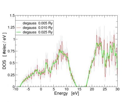
    degauss=0.025  !  [Ry]  broadening parameter
    fildos = 'dos_diamond_0.025Ry.dat'
 / 

The variable degauss controls the gaussian broadening used to approximate Dirac delta's in the calculation.

Try to change this value to get a feeling of the effect is has on the computed DOS.

An example is show in the figure below.

Band structure of Diamond

In order to compute a band structure we need to run a dedicated nscf calculation.

This will overwrite previous nscf calculations, but does not modify the previously compute density.

We need now to write the input file for a non-self consistent calculation using a regular k-point grid. The input file looks like:

 >$ cat nscf_bands.in
 &CONTROL
   calculation="bands"
   verbosity="high"     # not strictly needed but useful sometimes
   [...]
 /
 &SYSTEM
   alat=...
   ecutwfc=...
   nbnd=20              # let's include some empty states
 /
 [...]
 K_POINTS {crystal_b}
 6
 0.500  0.500  0.000   40    # X 
 0.000  0.000  0.000   40    # G 
 0.500  0.500  0.500   40    # L 
 0.750  0.500  0.250   40    # W 
 0.750  0.375  0.375   40    # K 
 0.000  0.000  0.000    1    # G

We run it as before

 mpirun -np 2 pw.x < nscf_bands.in > nscf_bands.out

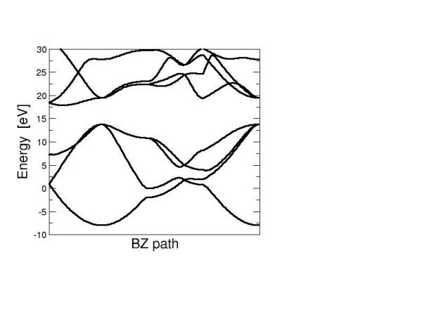
Next, bands can be reformatted for plotting using the bands.x provided by Quantum ESPRESSO.

Alternatively, the home-made tool

 ./LabQSM/tools/plot_bands.py  nscf_bands.out

can be used.

The resulting plot is reported below.