Solution LAB1 ecutwfc convergence 2
- Back to the previous page: Structural and electronic properties of semiconductors and metals #Convergences
Convergence of total energy differences wrt the kinetic energy cutoff
Use the same machinery (script to run the calculations, scripts to extract data from the output file) developed for the previous exercise, Solution to Exercise 3.
There we have been running calculations for alat=6.741. Let's pick a lattice variation, say 2%.
Change the script to run with such a modified parameter. For instance:
 #
 # set vars
 #
 stretch=0.01
 alat0=6.741
 alat=`echo $alat0 $stretch | awk '{ print $1*(1.0+$2)}'`
 nk=8
(of course it is also possible to just change the hardcoded alat value in the script).
It is also important to change the input and output filenames, e.g. modifying label:
 #
 label="nk${nk}_stretch${stretch}_ecut${ecutwfc}"
 #
We are now in the position to run the calculations for the new system for a range of ecutwfc values. Using the same script of Ex3 to extract the data,
$> ./extract.sh scf*stretch*.out > data_stratch
we obtain:
 $>  cat data_stretch.dat
 #  ecut [Ry]   etot [Ry]   time [sec]
 20.0000  -22.21905831   0.23
 30.0000  -22.53626807   0.32
 40.0000  -22.69832895   0.33
 50.0000  -22.75526586   0.92
 60.0000  -22.77763941   1.00
 80.0000  -22.79383663   1.21
 100.0000  -22.79691290   1.66
 120.0000  -22.79774354   3.56
 140.0000  -22.79794454   6.42
 160.0000  -22.79800726   5.32
 200.0000  -22.79802688   7.79
 300.0000  -22.79802865   21.11     # these last values are largely overconverged
 400.0000  -22.79802704   22.84     # just reported for completeness
Using the command paste we place side by side the results obtained in Ex3 without stretching and those
that we have just computed.
 $>  paste data.dat data_stretch.dat
 #  ecut [Ry]   etot [Ry]   time [sec]	#  ecut [Ry]   etot [Ry]   time [sec]
 20.0000  -22.20777973   0.19	  20.0000  -22.21905831   0.23
 30.0000  -22.53632376   0.33	  30.0000  -22.53626807   0.32
 40.0000  -22.70012158   0.41	  40.0000  -22.69832895   0.33
 50.0000  -22.75832711   0.97	  50.0000  -22.75526586   0.92
 60.0000  -22.78070087   1.16	  60.0000  -22.77763941   1.00
 [...]
This is convenient to use awk to compute the line-by-line difference of fields $5 and $2 (total energies w/ and w/o stretching):
 $>  paste data.dat data_stretch.dat | awk '{print $1, $5-$1}'
 # 0
 20.0000  -0.0112786
 30.0000   5.569e-05
 40.0000   0.00179263
 50.0000   0.00306125
 60.0000   0.00306146
 80.0000   0.00333661
100.0000   0.00331713
120.0000   0.00333176
140.0000   0.0033299
160.0000   0.00333089
200.0000   0.0033337
300.0000   0.00333215
400.0000   0.0033342
- Independently of the stretching parameter chosen, the accuracy of the difference is smaller that 0.0001 Ry for ecutwfc values larger than 80 Ry,
- Instead, we had to go for much larger values (120-150 Ry) to converge the absolute values of the total energies.
- We are indeed exploiting a form of error cancellation, due to the fact that what causes the total energy to converge slowly wrt ecutwfc are the oscillations of the wfcs and density in the region close to the nuclei.
- Fortunately, when changing the lattice parameter, such contributions do not affect the bonding, and, in turn, the energy difference between the two structures, thereby not showing up in the total energy differences.
- A similar situation happens also for total energy derivatives wrt to atomic positions (forces) or lattice parameters (stresses).
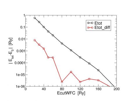
In the following graph we plot the data in log scale to compare with the convergence of the bare total energy.
IMPORTANT: in both cases we plot the absolute value of the E-E0, where E0 is the converged value (here taken as the value compute at 400 Ry ecutwfc).
- This means that we are plotting in log scale how much each quantity is changing because of the energy cutoff.
- As discussed above, the total energy difference is better behaved in terms of absolute convergence (the red curve is somehow shifted down wrt the black one).
- While it has a more noisy shape as compared to the total energy plot.
This last point can be understood by looking at the actual number of G-vectors used in the calculations.
- The number of G-vectors changes because of the ecutwfc variable.
- Dealing with two different lattice values, the set of G-vectors is actually different: we are using a different Fourier basis.
- When changing ecutwfc, dealing with two different basis introduces some noise.
For the sake of completeness, here we report the actual number of G-vectors used in the calculations for the two values of the lattice parameter.
 # ecut     Ng_latt1   Ng_latt2
  20.0000     941        941
  30.0000    1687       1807
  40.0000    2685       2733
  50.0000    3695       3719
  60.0000    4909       4957
  80.0000    7391       7631
 100.0000   10417      10777
 120.0000   13635      14067
 140.0000   17153      17573
 160.0000   20875      21595
 200.0000   29363      30347
 300.0000   53977      55369
 400.0000   82723      85275
which can be extracted by using a script alike the following:
 #!/bin/bash
 #
 file_list=$*
 output="#  ecut [Ry]   Ng"

 for file in $file_list
 do
   ecutwfc=`grep "kinetic-energy cutoff" $file | awk '{print $(NF-1)}'`
   gvec=`grep "FFT" $file | awk '{print $3}'`
   output="$output
   $ecutwfc  $gvec"
 done
 echo "$output" | sort -n
